In my previous article, you learned Python fundamentals. I also introduced the basic data structures. You can imagine you need more advanced data structures for analyzing SQL Server data, which comes in tabular format. In Python, there is also the data frame object, like in R. It is defined in the pandas library. You communicate with SQL Server through the pandas data frames. But before getting there, you need first to learn about arrays and other objects from the numpy library.
In this article, you will learn about the objects from the two of the most important Python libraries, namely, as mentioned, numpy and pandas.
A Quick Graph Demo
For a start, let me intrigue you by showing some analytical and graphic capabilities of Python. I am explaining the code just briefly in this section; you will learn more about Python programming in the rest of this article. The following code imports necessary libraries for this demonstration.
import numpy as np
import pandas as pd
import pyodbc
import matplotlib.pyplot as plt
Then we need some data. I am using the data from the AdventureWorksDW2016 demo database, selecting from the dbo.vTargetMail view.
Before reading the data from SQL Server, you need to perform two additional tasks. First, you need to create a login and a database user for the Python session and give the user the permission to read the data. Then, you need to create an ODBC data source name (DSN) that points to this database. In SQL Server Management Studio, connect to your SQL Server, and then in Object Explorer, expand the Security folder. Right-click on the Logins subfolder. Create a new login and a database user in the AdventureWorksDW2016DW database and add this user to the db_datareader role. I created a SQL Server login called RUser with password Pa$$w0rd, and a user with the same name.
After that, I used the ODBC Data Sources tool to create a system DSN called AWDW. I configured the DSN to connect to my local SQL Server with the RUser SQL Server login and appropriate password and change the context to the AdventureWorksDW2016 database. If you’ve successfully finished both steps, you can execute the following Python code to read the data from SQL Server.
# Connecting and reading the data
con = pyodbc.connect('DSN=AWDW;UID=RUser;PWD=Pa$$w0rd')
query = """SELECT CustomerKey, Age,
             YearlyIncome, TotalChildren,
             NumberCarsOwned
           FROM dbo.vTargetMail;"""
TM = pd.read_sql(query, con)
You can get a quick info about the data you read with the following code:
# Get the information
TM.head(5)
TM.shape
The code shows you the first five rows and the shape of the data you just read.
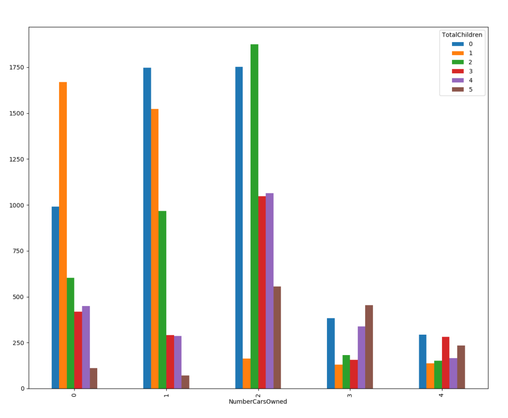
Now I can do a quick crosstabulation of the NumberCarsOwned variable by the TotalChildren variable.
# Crosstabulation
obb = pd.crosstab(TM.NumberCarsOwned, TM.TotalChildren)
obb
And here are the first results, a pivot table of the afore mentioned variables.
| TotalChildren NumberCarsOwned | 0 | 1 | 2 | 3 | 4 | 5 |
| 0 | 990 | 1668 | 602 | 419 | 449 | 110 |
| 1 | 1747 | 1523 | 967 | 290 | 286 | 70 |
| 2 | 1752 | 162 | 1876 | 1047 | 1064 | 556 |
| 3 | 384 | 130 | 182 | 157 | 339 | 453 |
| 4 | 292 | 136 | 152 | 281 | 165 | 235 |
Let me show the results of the pivot table in a graph. I need just the following two lines:
# Bar chart
obb.plot(kind = 'bar')
plt.show()
You can see the graph in the following figure.
Using the NumPy Data Structures and Methods
NumPy is short for Numerical Python; the library name is numpy. The library provides arrays with much more efficient storage and faster work than basic lists and dictionaries. Unlike basic lists, numpy arrays must have elements of a single data type. The following code imports the numpy package with alias np. Then it checks the version of the library. Then the code creates two one-dimensional arrays from two lists, one with implicit element data type integer, and one with explicit float data type.
# Numpay intro
np.__version__
np.array([1, 2, 3, 4])
np.array([1, 2, 3, 4], dtype = "float32")
You can create multidimensional arrays as well. The following code creates three arrays with three rows and five columns, one filled with zeroes, one with ones, and one with the number pi. Note the functions used for populating arrays.
np.zeros((3, 5), dtype = int)
np.ones((3, 5), dtype = int)
np.full((3, 5), 3.14)
For the sake of brevity, I am showing here only the last array.
array([[ 3.14,  3.14,  3.14,  3.14,  3.14],
       [ 3.14,  3.14,  3.14,  3.14,  3.14],
       [ 3.14,  3.14,  3.14,  3.14,  3.14]])
There are many additional functions that help you populating your arrays. The following code creates four different arrays. The first line creates a linear sequence of numbers between 0 and 20 with step 2. Note that the upper bound 20 is not included in the array. The second line creates uniformly distributed numbers between 0 and 1. The third line creates ten numbers between with standard normal distribution with mean 0 and standard deviation 1. The fourth line creates a 3 by 3 matrix of uniformly distributed integral numbers between 0 and 9.
np.arange(0, 20, 2)
np.random.random((1, 10))
np.random.normal(0, 1, (1, 10))
np.random.randint(0, 10, (3, 3))
Again, for the sake of brevity, I am showing only the last result here.
array([[0, 1, 7],
       [5, 9, 4],
       [5, 5, 6]])
In order to perform some calculations on array elements, you could use mathematical functions and operators from the default Python engine, and operate in loops, element by element. However, the numpy library includes also vectorized version of the functions and operators, which operate on vectors and matrices as a whole, and are much faster than the basic ones. The following code creates a 3 by 3 array of numbers between 0 and 8, shows the array, and then calculates the sinus of each element using a numpy vectorized function.
# Numpy vectorized functions
x = np.arange(0, 9).reshape((3, 3))
x
np.sin(x)
And here is the result.
array([[0, 1, 2],
       [3, 4, 5],
       [6, 7, 8]])
array([[ 0.        ,  0.84147098,  0.90929743],
       [ 0.14112001, -0.7568025 , -0.95892427],
       [-0.2794155 ,  0.6569866 ,  0.98935825]])
Numpy includes also vectorized aggregate functions. You can use them for a quick overview of the data in an array, using the descriptive statistics calculations. The following code initializes an array of five sequential numbers:
# Aggregate functions
x = np.arange(1,6)
x
Here is the array:
array([1, 2, 3, 4, 5])
Now you can calculate the sum and the product of the elements, the minimum and the maximum, the mean and the standard deviation:
# Aggregations
np.sum(x), np.prod(x)
np.min(x), np.max(x)
np.mean(x), np.std(x)
Here are the results:
(15, 120)
 (1, 5)
(3.0, 1.4142135623730951)
In addition, you can also calculate running aggregates, like running sum in the next example.
# Running totals
np.add.accumulate(x)
The running sum result is here.
array([ 1, 3, 6, 10, 15], dtype=int32)
There are many more operations on arrays available in the numpy module. However, I am switching to the next topic in this Python learning tour, to the pandas library.
Organizing Data with Pandas
The pandas library is built on the top of the numpy library. Therefore, in order to use pandas, you need to import numpy first. The pandas library introduces many additional data structures and functions. Let’s start our pandas tour with the panda Series object. This is a one-dimensional array, like numpy array; however, you can define explicitly named index, and refer to that names to retrieve the data, not just to the positional index. Therefore, a pandas Series object already looks like a tuple in the relational model, or a row in a table. The following code imports both packages, numpy and pandas. Then it defines a simple pandas Series, without an explicit index. The series looks like a simple single-dimensional array, and you can refer to elements through the positional index.
# Pandas series
ser1 = pd.Series([1, 2, 3, 4])
ser1[1:3]
Here are the results. I retrieved the second and the third element, position 1 and 2 with zero-based positional index.
1    2
2    3
Now I will create a series with explicitly named index:
# Explicit index
ser1 = pd.Series([1, 2, 3, 4],
                 index = ['a', 'b', 'c', 'd'])
ser1['b':'c']
As you could see from the last example, you can refer to elements using the names of the index, which serve like column names in a SQL Server row. And below is the result.
b    2
c    3
Imagine you have multiple series with the same structure stacked vertically. This is the pandas DataFrame object. If you know R, let me tell you that it looks and behaves like the R data frame. You use the pandas DataFrame object to store and analyze tabular data from relational sources, or to export the result to the tabular destinations, like SQL Server. When I read SQL Server data at the beginning of this article, I read the tabular data in a Python data frame. The main difference, compared to a SQL Server table, is that a data frame is a matrix, meaning that you still can refer to the data positionally, and that the order of the data is meaningful and preserved.
Pandas data frame is a very powerful object. You have already seen the graphic capabilities of it in the beginning of this article, when I created a quite nice bar chart. In addition, you can use other data frame methods to get information about your data with help of descriptive statistics. He following code shows how to use the describe() function on the whole data frame to calculate basic descriptive statistics on every single column, and then how to calculate the mean, standard deviation, skewness, and kurtosis, i.e. the first four population moments, for the Age variable.
# Descriptive statistics
TM.describe()
TM['Age'].mean(), TM['Age'].std()
TM['Age'].skew(), TM['Age'].kurt()
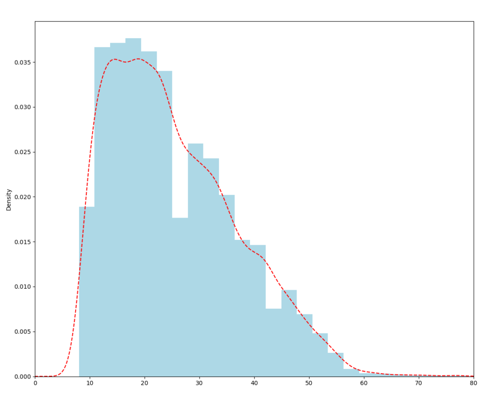
Let me finish this article with another fancy example. It is quite simple to create even more complex graphs. The following code shows the distribution of the Age variable in histograms and with a kernel density plot.
# Another graph
(TM['Age'] - 20).hist(bins = 25, normed = True,
                      color = 'lightblue')
(TM['Age'] - 20).plot(kind='kde', style='r--', xlim = [0, 80])
plt.show()
You can see the results in the following figure. Note that in the code, I subtracted 20 from the actual age, to get slightly younger population than exists in the demo database.
Conclusion
I guess the first article in this series about Python was a bit dull. Nevertheless, you need to learn the basics before doing anything fancier. I hope that in this article you got more intrigued by the Python capabilities for working on data. In the forthcoming articles, I will go deeper into the graphing capabilities and in data science with Python.
Read the whole series:
Python for SQL Server Specialists Part 1: Introducing Python
Python for SQL Server Specialists Part 3: Graphs and Machine Learning
Python for SQL Server Specialists Part 4: Python and SQL Server
This is just an introduction, for more on starting with data science in SQL Server please refer to the book “Data Science with SQL Server Quick Start Guide” (https://www.packtpub.com/big-data-and-business-intelligence/data-science-sql-server-quick-start-guide), where you will learn about tools and methods not just in Python, but also R and T-SQL.
