Suppose that a large car rental company needs to track each customer contract, which is represented by a row in a database table. Each row includes the customer’s identifier and a pair of dates delimiting the rental time period. A SQL request to find all contracts effective between two dates might end up scanning a large portion of the table because interval intersection queries generally have no built-in support in a relational database management system (RDBMS).
In the year 2000, a group of German researchers—Hans-Peter Kriegel, Marco Pötke, and Thomas Seidl from the Institute for Computer Science at the University of Munich—invented the Relational Interval Tree (RI-Tree), an extremely ingenious structure to efficiently handle interval queries in SQL. They wrote about it in the paper “Managing Intervals Efficiently in Object-Relational Databases”.
However, one aspect of the RI-Tree is a bit tricky: There is no simple way to handle batched insertion (i.e., INSERT SELECT statements) because each inserted row might modify the value of one of the tree’s four parameters. This article covers a variant of the RI-Tree, the Static RI-Tree, which supports batched insertion with excellent performance.
The original RI-Tree has four associated parameters: offset, leftRoot, rightRoot, and minstep. The function of these parameters is to save CPU time by controlling the tree’s height, thereby avoiding many useless iterations while traversing the tree. Unfortunately, the insertion of an interval is dependent on these parameters, which in turn, might be modified by the insertion itself. This makes writing an INSERT SELECT statement difficult. The Static RI-Tree does not use any of the original parameters. Instead, a newly inserted interval is dependent only on row data, which makes using an INSERT SELECT statement feasible. Consequently, this tree covers the entirety of the data space all the time. No dynamic expansion takes place, hence the name Static RI-Tree. Because this new variant is static, it traverses the tree in a different way than the original RI-Tree to avoid the many iterations just mentioned.
The static RI-Tree
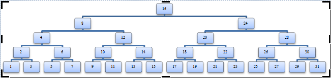
The backbone of the Static RI-Tree is implemented the same as a binary tree: with its nodes labeled as integer numbers from 1 through 2^(N-1) in order (where N is the size of the integer data type used, in bits). The value of the root is set to 2^(N-1). You can use dates instead of integers by providing a simple mapping between dates and integers. Figure 1 shows a sample binary tree in which N = 5.
The fork node plays a crucial role in the structure because it determines where an interval is inserted into the Static RI-Tree. Its value is used in the node column of the Intervals table, as shown in Listing 1. Also shown in this code are the two indexes built on this table, as in the original RI-Tree.
Assuming an interval [lower, upper], with lower and upper being integers, the fork node is defined as the topmost node w in the following relation: lower <= w <= upper. As described in the original paper, the forkNode function proceeds by iterating through the tree from the root down to the fork node, as shown in Listing 2.
CREATE TABLE Intervals
(
id INT NOT NULL PRIMARY KEY,
node INT NOT NULL, -- Computed as forkNode(lower, upper)
lower INT NOT NULL,
upper INT NOT NULL
);
CREATE INDEX lowerIndex ON Intervals(node, lower);
CREATE INDEX upperIndex ON Intervals(node, upper);
FUNCTION int forkNode(int lower, int upper) {
int node = 2N-1;
for(int step = node/2; step >= 1; step /= 2)
if upper < node
node -= step;
else if node < lower
node += step;
else
break;
return node;
}
The forkNode function iterates through the tree to the fork node. The fork node plays a crucial role because it determines where an interval is inserted into the tree
The Problem
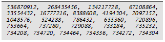
With this simplified implementation, there is a problem: The number of iterations needed in a call to forkNode depends on the tree’s height and can waste many CPU cycles. For instance, suppose we are using 32-bit signed integers that are positive numbers ranging from 1 through 2^(31-1) = 2147483647. If we call forkNode with the interval [734288, 734317], the function starts at the root, whose value is 2^(30) = 1073741824, then steps through the following nodes:
A New Way of Finding the Fork NodeFor the remainder of this article, let nx represent a node of the tree with value x. Let us assume we are searching the fork node for an interval [lower, upper] in which nlower is the node with the value of lower and nupper is the node with the value of upper. Looking closely at the sample binary tree in Figure 1, notice that the fork node can be determined from lower and upper alone. Instead of starting from the root, we can walk up the tree from both nlower and nupper until we reach their lowest common ancestor. This will be the fork node. To demonstrate that the lowest common ancestor of nlower and nupper is indeed their fork node, consider the following cases:
- Case 1: If nlower and nupper have a lowest common ancestor of nx, which is neither nlower nor nupper, then nlower will be in nx’s left subtree and nupper will be in nx’s right subtree. As such, x is in the interval [lower, upper]. Because the value of any ancestor of nx is outside this interval, nx is the fork node.
- Case 2: If nlower = nupper, the fork node is that node. It is also the lowest common ancestor.
- Case 3: If nlower is an ancestor of nupper, the fork node will be nlower because it is the highest node whose value is contained in the interval [lower, upper], while all of its ancestors are outside this interval. Also, nlower is the lowest common ancestor.
- Case 4: If nupper is an ancestor of nlower, the fork node will be nupper for reasons symmetric to those of Case 3.
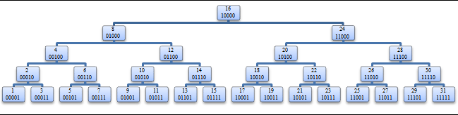
We now need a method to compute the fork node efficiently from lower and upper. The sample binary tree in Figure 2 has its nodes labeled with their decimal and binary values. Looking at the binary values of the integers in the tree, we can make several interesting observations:
- Observation 1: For any non-leaf node possessing an even value, the binary representation of this value will have a non-empty sequence of trailing 0 bits, whose number depends on the height of the node in the tree. Let us call L the sequence of leading bits before these trailing 0 bits. L uniquely identifies a non-leaf node.
- Observation 2: Assume we have a non-leaf node nx with a leading bit sequence of L. In nx’s left subtree, the prefix of the value of any node is L with its rightmost 1 bit cleared. In nx’s right subtree, the prefix of the value of any node is L.
- Observation 3: Assume we have a non-leaf node nx. The node nx-1 belongs to the left subtree of nx (assuming that the value 0 is allowed in the tree). Because the fork node of interval [x, y] (where x <= y) is nx or an ancestor of nx, the interval [x-1, y] has the same fork node. This allows the replacement of x with x-1 without changing the resulting fork node.
- Observation 4: Assume we have a leaf node nz. The last bit of z is set to 1 because it is the value of a leaf node. In this case, z-1 will have the exact same bit representation as z, except for the last bit, which is set to 0.
These observations enable us to define a method to compute the fork node directly from nlower and nupper. Using these observations, let us examine the four cases previously mentioned and then incorporate the ideas into one general method. In Case 2, when nlower is a non-leaf node, Observation 3 tells us that the leading sequence L can be computed as the leftmost matching bits of lower-1 and upper with a “1” bit appended. When nlower is a leaf node, consider the following: Because Observation 4 applies and lower = upper, lower-1 differs from upper on the last bit only. Therefore, the leftmost matching bits of lower-1 and upper with a “1” bit appended equals lower and upper, which is also the fork node. In Cases 1, 3, and 4, when nlower is a non-leaf node, Observation 3 tells us that the leading sequence L can be computed as the leftmost matching bits of lower-1 and upper with a “1” bit appended. If nlower is a leaf node, consider the following: Because Observation 4 applies, lower-1 is the only value differing from lower exclusively on the last bit. Also, because lower-1 < lower, then lower-1 ≠ upper. Further, because lower < upper, lower differs from upper on another bit than the last. As a consequence, the last bit of lower is irrelevant in the determination of the fork node, so lower can be replaced by lower-1. To conclude, the computation of the fork node boils down to:
- Finding the sequence of leftmost matching bits between lower-1 and upper.
- Appending a “1” bit.
- Filling the remaining right bits with 0’s.
Let us investigate a couple of examples:
- Example 1: In the tree represented in Figure 2, we are looking for the fork node of the interval [5, 10]. This is Case 1, and the fork node is 8. Let us replace 5 with 4, examine the binary representations of 4 and 10, and search for the leftmost matching bits. The search reveals a sequence reduced to one 0 bit. The leading sequence of the fork node is thus L = 01. This leading sequence uniquely identifies the node labeled 8.
- Example 2: Let us find the fork node of the interval [12, 15]. This is Case 3, and the fork node is 12. Replace 12 with 11, examine the binary representations of 11 and 15, and search for the leftmost matching bits. The search reveals the sequence 01. After appending a “1” bit, we get the leading sequence L = 011, which corresponds to the node labeled 12.
- Example 3: We are now looking for the fork node of the interval [21, 24]. This is Case 4, and the fork node is 24. Replace 21 with 20, examine the binary representations of 20 and 24, and search for the leftmost matching bits. The search reveals the sequence 1. After appending a “1” bit, we get the leading sequence L = 11, which corresponds to the node labeled 24.
- Example 4: Let us find the fork node of the interval [21, 21]. This is Case 2, and the fork node is 21. Replace 21 with 20, examine the binary representations of 20 and 21, and search for the leftmost matching bits. The search reveals the sequence 1010. After appending a “1” bit, we get the leading sequence L = 10101, which corresponds to the node labeled 21.
A Better forkNode functionLet us use the new method just outlined to rewrite the forkNode function and attempt to cut back on iterations. This requires knowledge of the integers’ storage size. Listing 3 shows the new implementation of the forkNode function for 32-bit integers.
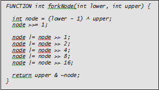
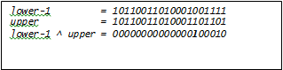
This looks strange, doesn’t it? Let’s analyze the logic. In the int node = (lower – 1) ^ upper instruction, the ^ operator is used to compute an exclusive bitwise OR operation between lower-1 and upper. This helps find the leftmost sequence of matching bits between lower-1 and upper because the exclusive OR clears out those bits, while the leftmost 1 bit in the result indicates the position of the leftmost non-matching bit between lower-1 and upper. Let us call this position w. For example, Figure 3 shows the result of this instruction when lower = 734288 and upper = 734317.
The >> operator shifts all bits to the right by the number of positions indicated by the number appearing after the operator. So, the node >>= 1 instruction shifts the value of the node variable 1 bit to the right (to position w + 1) and assigns the result to node. At this point, the result is:

The series of five node |= node >> n instructions copies the 1 bit at position w+1 to the right until all bits at the right of position w+1 are set to 1. In our example, these five instructions produce the result:

The ~ operator negates all bits: 0’s are converted to 1’s and 1’s to 0’s. This is to prepare a bitmask to zero-out all bits after position w. In our example, this yields:

The final return upper & ~node instruction applies the bitmask to upper to clear out the bits and form the leading sequence with 0’s appended. This corresponds to the fork node. In this case, the result is:

This implementation is a significant optimization because the number of instructions executed is constant and much smaller for many intervals [lower, upper]. CPU time is being saved.
A Set-Based Intersection Query
In the original RI-Tree, the approach to filling the leftNodes and rightNodes tables is an iterative algorithm traversing the binary tree from the root to the fork node, then from the fork node to the nodes closest to nlower and nupper. In each iteration, the algorithm might insert a row into the leftNodes or rightNodes table. Although these tables are small, an RDBMS would typically proceed much faster with a set-based computation of these tables.
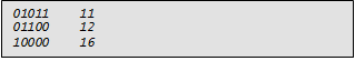
Let us look for a replacement for the iterative fill-up of the leftNodes and rightNodes tables. Instead of proceeding from the root of the tree down to the nlower and nupper nodes, let us go in the opposite direction—from nlower and nupper up to the root. What happens to the binary value of a node during this process? Each step up the tree clears the rightmost 1 bit and sets the bit to its left to 1 if it was not set already. For instance, going from node 11 to node 16 in Figure 2 involves the following steps:
01011 11
01010 10
01100 12
01000 8
10000 16
To populate the leftNodes and rightNodes tables from the bottom up, we need to separate values into two groups: values smaller than the bottom node’s value and values greater than the bottom node’s value. To find values smaller than the bottom node’s value, we just need to clear the rightmost 1 bit. To find values greater than the bottom node’s value, we need to clear the rightmost 1 bit, set the rightmost 0 bit to its left, and clear all the bits in between. In our example above of going from node 11 up to node 16, this strategy yields the following values smaller than 11:

And the following values greater than 11:
To implement these bit manipulations, we will use the BitMasks table. Listing 4 shows the code to create this table.
CREATE TABLE BitMasks
(
b1 INT NOT NULL,
b2 INT NOT NULL,
b3 INT NOT NULL
);
Assuming N represents the size of the integer data type in bits, the BitMasks table is filled with N-1 rows. Let us call r the row index, ranging from 1 through N-1. The column b1 is computed by clearing the r rightmost bits and setting the other bits. One easy way to generate b1 values is to use –(2r). Column b2 is computed by setting bit r (where bits are counted from right to left) and clearing all other bits. This can be computed as 2r-1. Column b3 is computed as b2 * 2. For instance, Table 1 shows the binary values when N = 5.
Table 1 Sample BitMasks table
Note that in the following explanation of the BitMasks table, the bitwise AND operator and the bitwise OR operator are represented by the & and | characters, respectively.
Assuming we want to retrieve all ancestors of node nx that have a value smaller than x or all ancestors of node nx that have a value greater than x, x will be combined with all rows of the BitMasks table. All parent nodes of nx that have a value smaller than x are nodes with a value equal to x & b1 where x & b2 is different from 0. Similarly, all parent nodes of nx that have a value greater than x are nodes with a value equal to (x & b1) | b3 where x & b3 is equal to 0. Thus, the SQL code required to populate the leftNodes and rightNodes tables will be that shown in Listing 5.
Listing 5 SQL code to populate the leftNodes and rightNodes tables
Implementing the Static RI-Tree with SQL Server
I initially implemented the optimized forkNode function using Microsoft SQL Server 2008 and T-SQL. I added the node column to the Intervals table as a computed, persisted column whose formula calls up the forkNode function, as shown in Listing 6. This worked well and the processing time of INSERT SELECT statements was significantly reduced compared to the iterative forkNode implementation.
Listing 6 The Intervals table with node as a computed column
Much better performance could be achieved by converting forkNode to a CLR user-defined function and storing the .NET assembly in the database. However, not everyone is familiar with .NET, and some companies forbid the use of CLR code. Fortunately, in this case, we can achieve performance close to that of a .NET function in T-SQL. All that is needed is an optimized formula written directly into the computed column definition of the CREATE TABLE statement. This has the additional benefit of eliminating the need for a call to the forkNode function. (Function calls are expensive in terms of time.)
Clearing a series of rightmost bits can be achieved with modulo and subtraction operators. For instance, clearing the five rightmost bits of integer x can be written as x – x mod 25. Finding position w of the leftmost 1 bit can be done with the LOG and FLOOR functions. For instance, the position of the leftmost bit of integer x is Log2x. The fastest T-SQL implementation I could come up with is shown in Listing 7, which I tested on SQL Server 2008 and SQL Server 2005. This code probably looks strange, so let us analyze the logic.
Listing 7 The Intervals table with node as a computed column
The CREATE TABLE statement in Listing 7 uses T-SQL’s exclusive bitwise OR operator (^) and modulo operator (%). The expression POWER(2, FLOOR(LOG( (lower – 1) ^ upper)/LOG(2))) is equivalent to the mathematical expression 2^(⌊ log_2 ((lower-1) XOR upper)⌋, where the FLOOR function computes the greatest integer less than or equal to its operand, like the pair of mathematical operators ⌊and ⌋.
The expression upper % POWER(2… extracts the bits after position w and the full expression subtracts these bits from upper, in effect clearing them.
Insertion Testing Scripts
Let us compare the different implementations of forkNode in the Static RI-Tree. First, though, we need to create an auxiliary table that contains 10,000,000 numbers. The code to generate this table is shown in Listing 8. We also need to generate 10,000,000 random intervals in a staging table so that the different interval tables all use the same sample data. Listing 9 contains the code to create the staging table.
DECLARE @limit INT = 10000000, @cnt INT = 1;
CREATE TABLE dbo.Nums(n INT NOT NULL
PRIMARY KEY);
INSERT INTO dbo.Nums VALUES(1)
WHILE @cnt * 2 <= @limit
BEGIN
INSERT INTO dbo.Nums WITH(TABLOCK)
SELECT @cnt + n
FROM dbo.Nums (NOLOCK);
SET @cnt *= 2;
END
INSERT INTO dbo.Nums WITH(TABLOCK)
SELECT @cnt + n
FROM dbo.Nums (NOLOCK)
WHERE @cnt + n <= @limit;
Listing 9 Code to create the staging table
Listing 10 contains the script for creating and filling the traditional Intervals table. Also, a filler node column has been added so that rows occupy the same storage space as those of a Static RI-Tree. Thus, the insertion into the Intervals table establishes a baseline for performance. What we want for the other implementations is to get as close as possible to that baseline.
Listing 10 Code to create and fill the traditional Intervals table
Listing 11 contains the iterative implementation of the forkNode function. The code in Listing 12 creates the Intervals2 table, whose node column uses the iterative forkNode function. We expect the insertion into this table to be slow because T-SQL is fairly slow when executing loops.
Listing 11 The iterative implementation of the forkNode function
Table 2 Times observed when filling the interval tables
Listing 12 Code to create the Intervals2 table, which uses the iterative forkNode function
Listing 13 contains the optimized implementation of the forkNode function. The code in Listing 14 creates the Intervals3 table, whose node column uses the optimized forkNode function. The optimized implementation should be faster than the iterative implementation because no loop is used. Instead, the optimized function is encapsulated inside the forkNode body. This is useful for seeing the overhead of calling a user-defined function.
Listing 13 The optimized implementation of the forkNode function
Listing 14 Code to create the Intervals3 table, which uses the optimized forkNode function
Listing 15 contains a script to create the Intervals4 table, whose node column uses the optimized inline formula. We expect this implementation to be the fastest. Table 2 summarizes the amount of time it took to fill the tables. I obtained these times on my desktop computer, which is an Intel Core 2 Duo E8500 processor, working at 3.17 GHz, with 4GB RAM. SQL Server 2008 was installed and queried locally.
Listing 15 Code to create the Intervals4 table, which uses the optimized inline formula
A sample intersection query
Let us now compare the performance of an intersection query when using the traditional and Static RI-Tree approaches. Let us run a query that finds all intervals intersecting the interval [826216, 826254] in the Intervals table (traditional approach) and Intervals4 table (Static RI-Tree approach).
Traditional approach: Running the query against the Intervals table is very simple, as Listing 16 shows. However, SQL Server ends up scanning too much data because there isn’t an index setup that can make good use of both the @lower and @upper parameters. To remedy this situation, we can attempt to create useful indexes, as shown in Listing 17.
Listing 16 Traditional intersection query
Listing 17 Code to create indexes for the traditional intersection query
When we run the query again after the indexes are created, SQL Server creates an execution plan involving one of the indexes, basing its choice on the current stated values of @lower and @upper, as Figure 4 shows. It then reuses the plan in subsequent queries, even when the other index would have been more appropriate. This means there is no stable plan in the cache. Thus, even when using one of the indexes, SQL Server ends up scanning too much data. On my computer, this query involved 15,498 logical reads and consumed 358 milliseconds of CPU. (Typically, the RECOMPILE query hint can be used to improve this type of situation, but in this case, the query would not benefit from cached plans.)
Figure 4 The execution plan for the traditional intersection query
Static RI-Tree approach: Intersection queries using the Static RI-Tree approach involve the BitMasks table. Sample code for filling the BitMasks table is shown in Listing 18.
Listing 18 Filling the BitMasks table
Listing 19 shows the query that will be run against the BitMasks table. This is the same query used in the traditional approach, except it has been adapted for use with the Static RI-Tree. Before we can run this query, though, we need to create the indexes on the Intervals4 table using the code in Listing 20.
Listing 19 Static RI-Tree intersection query
Listing 20 Code to create indexes for the Static RI-Tree intersection query
For this query, SQL Server generates a stable execution plan, as shown in Figure 5. The great advantage of this plan is that it can be reused for all intersection queries because it does not depend on any selectivity. On my machine, this query involved 124 logical reads and consumed 0 milliseconds of CPU.
Note that, to favor code reuse, the leftNodes and rightNodes tables can be implemented as inline table-valued functions, which SQL Server expands at execution time (see Listing 21). In this instance, no additional performance penalty due to a function call is incurred. Listing 22 shows the intersection query using these functions.
Figure 5: The execution plan for the Static RI-Tree intersection query
Listing 21 The leftNodes and rightNodes tables implemented as inline table-valued functions
Listing 22 Static RI-Tree intersection query using the leftNodes and rightNodes functions
Conclusion
In this article, I presented the Static RI-Tree, which uses an INSERT SELECT statement to insert intervals in batches into the database with good performance. I also presented a way to enhance the performance of interval queries by using a set-based query instead of having to use procedural code with loops and iterations, which typically runs slower in an RDBMS.

Laurent Martin is a software architect working in Paris, France, for StatPro, a leading portfolio analysis and asset valuation provider. Laurent has been working in the software industry for over 20 years, specializing in Microsoft technologies.
Latest posts by lmartin (see all)
- Using the Static Relational Interval Tree with time intervals – June 27, 2013
- Advanced interval queries with the Static Relational Interval Tree – January 30, 2013
- A Static Relational Interval Tree – November 22, 2011
